
You can find me on Twitter @bhutanisanyam1
You can find the Markdown File Here
You can find the Lecture 1 Notes here
Lecture 2 Notes can be found here
Lecture 4 Notes can be found here
Lecture 5 Notes can be found here
These are the Lecture 3 notes for the MIT 6.S094: Deep Learning for Self-Driving Cars Course (2018), Taught by Lex Fridman.
All Images are from the Lecture Slides.
Here is a quick Primer if you want a brief intro to Reinforcement Learning
To what extent can we teach systems to perceive and act in this world from Data?
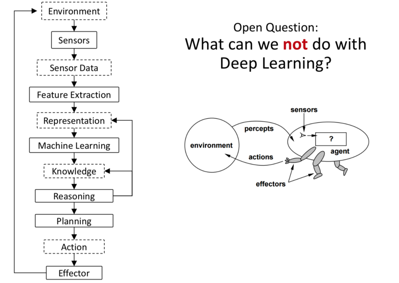
Stack of Tasks an AI System needs to perform
- Environment: World that the system is operating in.
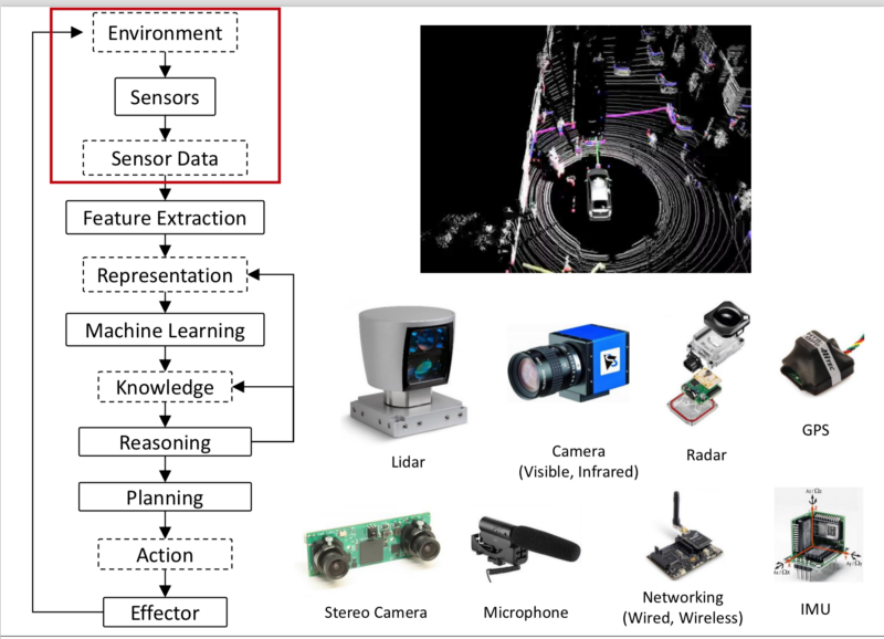
- Sensor: Sensed by sensors that take in the world and convert it to raw data that can be perceived by the machine. Input for robots operating in the world.
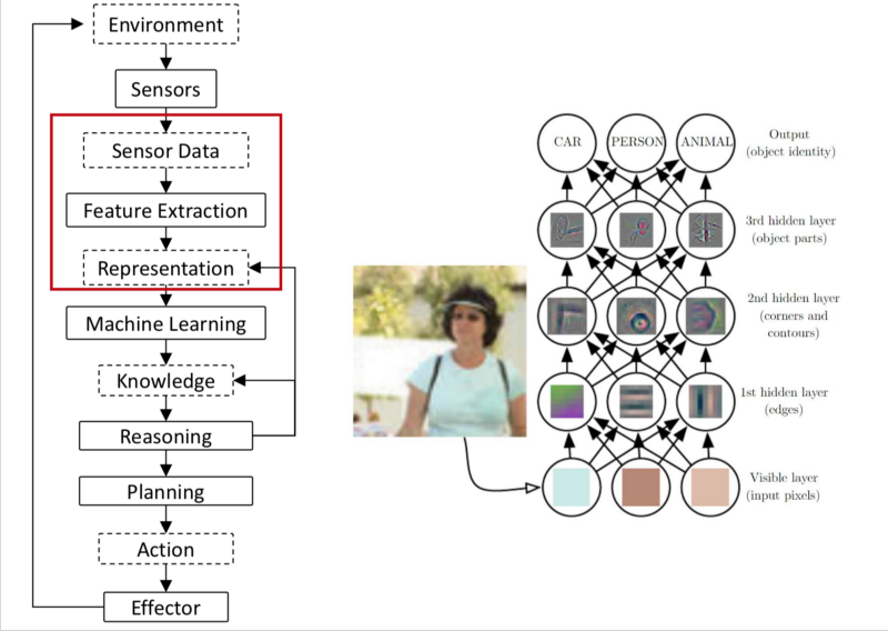
- Sensor Data: The raw data extracted by the sensors.
- Feature Extraction: Features are extracted from sensor data. Structure is extracted from the data such that you can input, discriminate, separate and understand the data.
The raw sensory data is processed, in multiple higher order abstractions. Deep Learning automates this task which was earlier performed by Human Experts. - We form higher order representations based on which ML techniques can be applied.
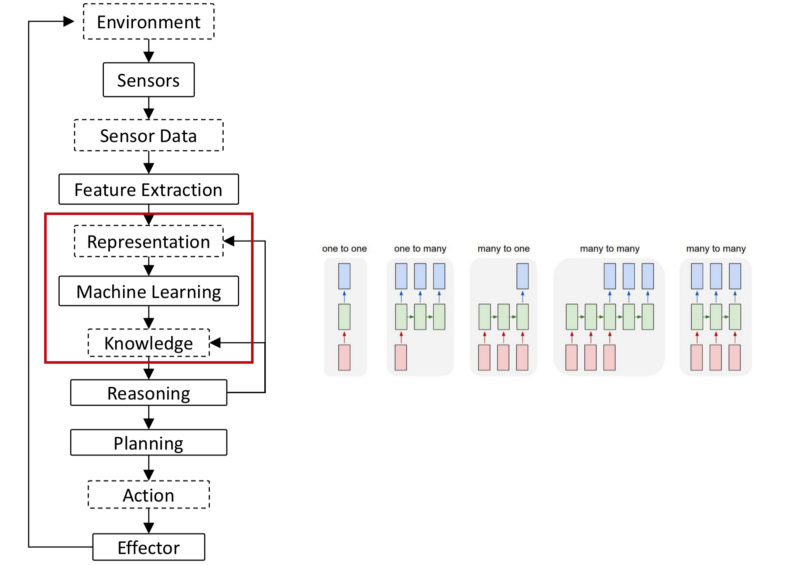
- Once ML techniques converts the data into simple actionable information, we aggregate that information into knowledge. The Deep Learning Networks are able to perform Supervised Learning tasks, Generative tasks, Unsupervised techniques. The knowledge, is simple & Clean usable values. These could be single values, speech, images, etcetra.
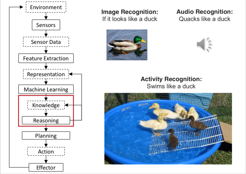
- We build a taxonomy, a library of knowledge. We connect the ideas.
- The agents reasons based on the taxonomy: Connects data from past and senses the world, defines a plan according to the Goal. (Goal, here could be Reward function).
Planning: Fusing the sensor information and making actions are more mendable to DL approach.
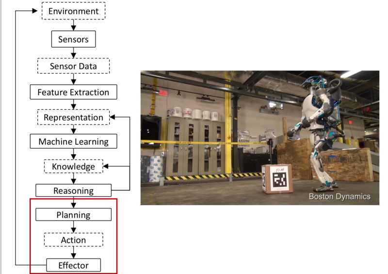
- Since it performs in the real world, it must have effectors that can act in the real world.
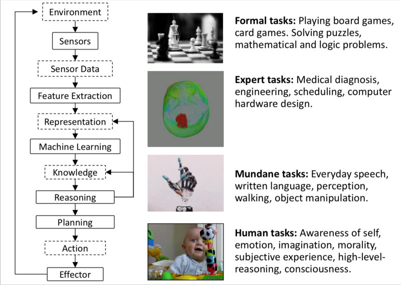
How Much of the AI Stack can be ‘Learned’?
We can learn the representation and knowledge. NN map the data to information, Kernel methods are effective here as well.
Mapping the data from right sensor data to knowledge is where DL Shines.
Open Question: Can We extend this to reasoning and actionable information end-to-end?
Q2, Can we extend this to real world cases of SDC and Robotics?
Types of Deep Learning
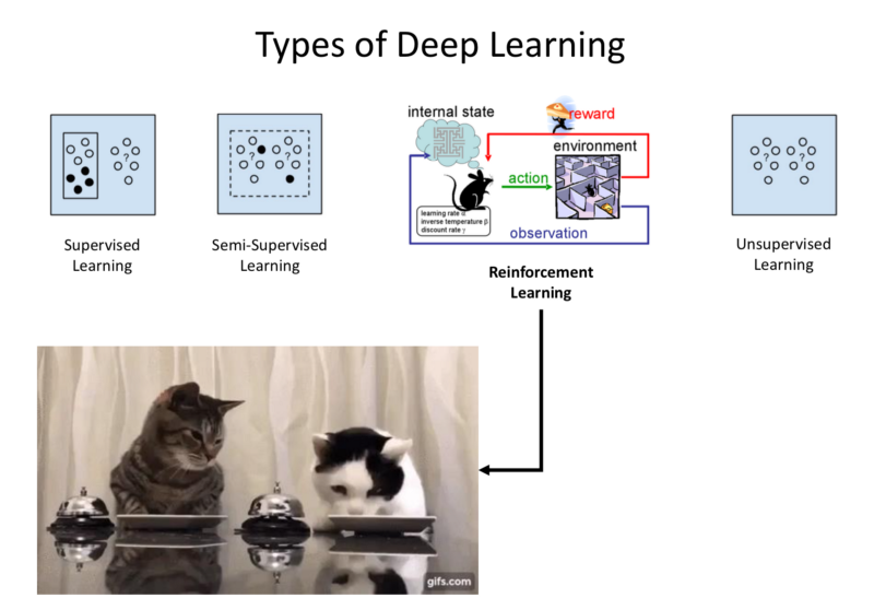
- Supervised: Every single data point is labelled by the humans.
- Unsupervised: Data is unlabelled.
- Semi-Supervised Learning: Some data is annotated by humans.
- Reinforcement Learning: RL is a subcategory of Semi-Supervised Learning.
Goal: Learn from sparse Reward/supervised data and take advantage of the fact that a temporal dynamics is followed from state to state, which can be propagated through time to infer knowledge about reality based on previous data. We can generalise the sparse learning information over real world.
Philosophical Motivation for Reinforcement Learning
Supervised Leanring: Memorization of Ground truth data in order to form representations that generalises from the ground truth.
Reinforcement Learning: Brute-Force propagate the sparse information through time to assign quality reward to state that does not directly have a reward. To make sense of the world when the data/reward is sparse, but are connected through time. This is equivalent of Reasoning.
Agent and Environment
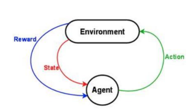
Connection through time is modelled as:
There is an agent, performing an action in the environment, receives a new state and a reward. This process continues over and over.
Examples:
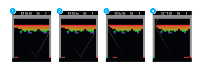
- Atari Breakout: Agent is the Paddle.
Each action that the agent takes has an influence on the evolution of the environment. The success is measured by summed reward mechanism. Here points are given by the game. The scheme must be normalised in a way that is interpretable by the system. The goal is to maximise the goal.
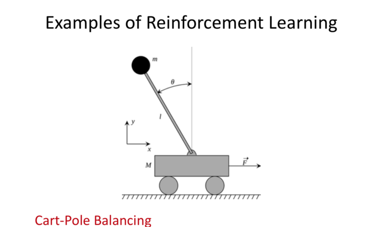
- Cart-Pole Balancing:
Goal: Continuous problem of balancing pole on top of moving cart.
State: Angle, angular verlocity, horizontal velocity of the cart.
Actions: Horizontal Force to the cart.
Reward: 1 at each time step if the pole is upright.
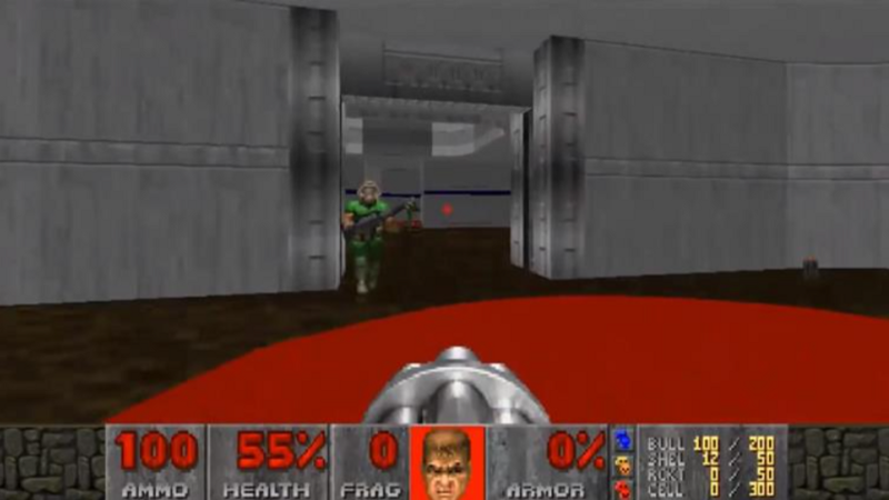
- All First person shooter games
Doom: Goal: Eliminate all opponents.
State: Raw Pixels from the game
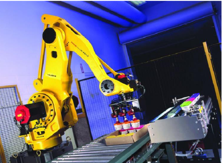
- Industrial Robotics:
Bin Packing using a robot.
Goal: Pick a box and put it into a container.
State: Raw Pixels of the world.
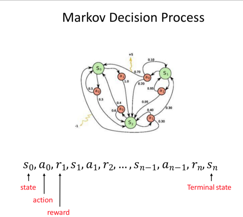
- Markov Decision Process: Action-Reward-State until terminal state is received.
Major Components of an RL Agent
1 or more of these:
- Policy: Plan of what kind of action to perform in every state.
- Value Function: Sense of what is a good state to be in and what is a good action that can be performed.
- Model: Agent’s representation of the World.
Ex: Robot in a room
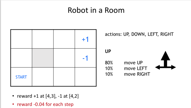
Deterministic approach: Shortest path is to be chosen.
Non-Deterministic
Key Observation: Every single state in the space must have a plan to control the non-deterministic environment.
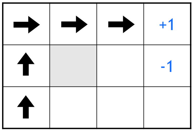
If reward function is designed such that every single step is penalised, the optimal policy in this case would be to chose the shortest path.
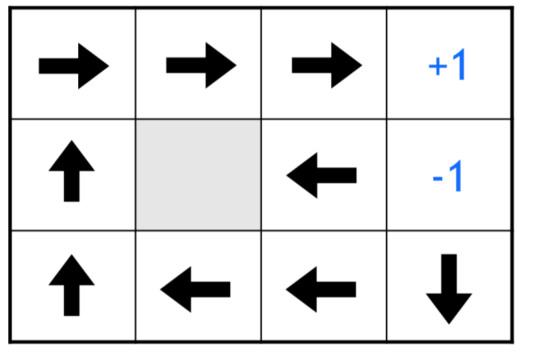
If we reduce the penalty, the randomness in movements is allowed.
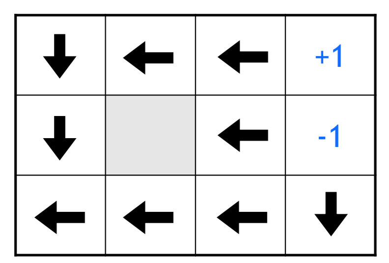
If we turn the reward to +ve to movement, there is an increased incentive for staying on the board without finishing.
Value Function:
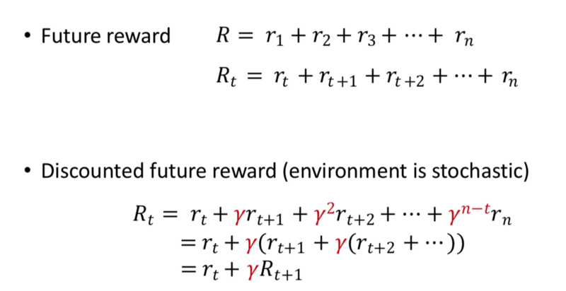
Value of the Environment state is the reward we are likely to receive in the future. This is determined by discounting the future discount.
Gamma: Reduces the importance of future goal.
A good strategy is maximising the sum of discounted future goals.
Q-Learning:
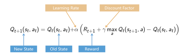
We use any policy to estimate state that maximises the future reward.
This allows us to consider much larger state space and action space.
We move about simulation taking actions and updating our estimate of how good actions are.
Exploration Vs Exploitation:
As a better estimate is formed of the Q-function, we form a better sense of the the better actions that can be performed. This is still not perfect so there is a value of Exploration. With improvements in estimation, the lesser the value for exploration.
So Initially we want to explore more and reduce that with time as our estimates become more accurate.
So the Final System, should operate in a greedy way according to the Q-Fucntion.
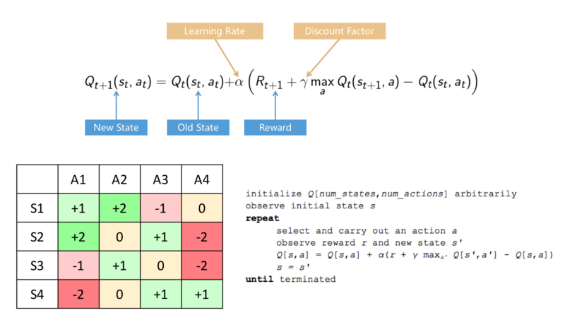
For tabular representation of Q-Function.
Y-Axis is states, X-Axis is Actions.
The table is initialised in a random manner and it is updated with the bellman equation, over time the approximation becomes the appropriate table.
Problem: When the Q-Table grows exponentially. Ex: Using Pixel inputs from real world/game. The potential state space, possible combinatorial states are larger than what System memory can hold, larger than what can be estimated using the Bellman Equation.
Deep RL:
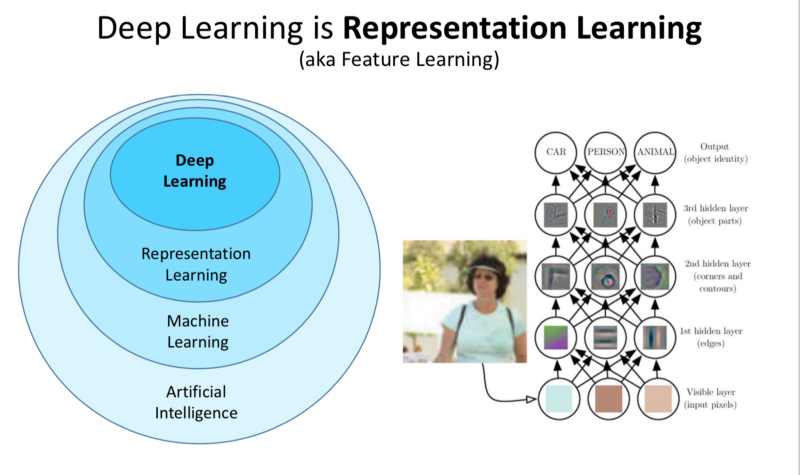
NN are really good at estimation.
DL: Allows us to approximate values over much larger state space as compared to ML. This allows us to deal with raw values of sensory data, it is much more capable to deal with real world applications; it is generalisable.
The understanding comes from converting the Raw sensory information to simple useful information based on which action can be taken.
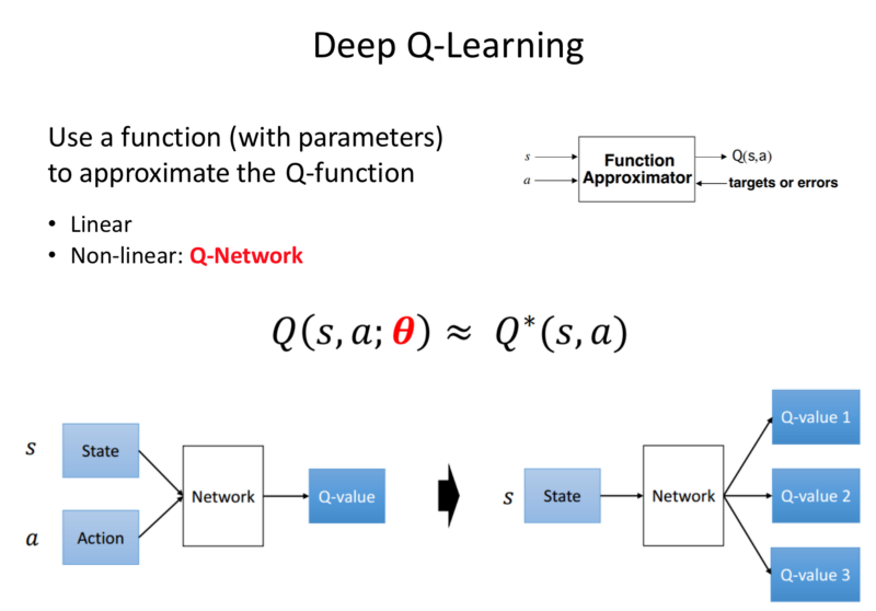
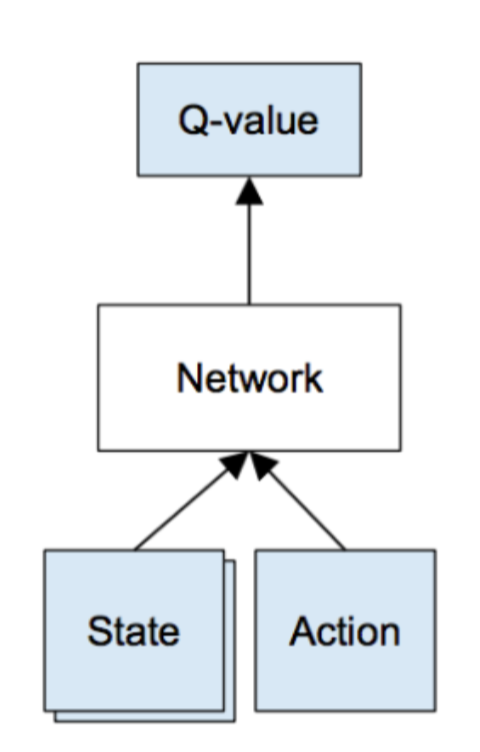
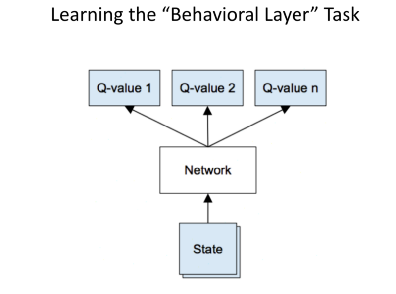
Instead of the Q-function, we plug in a NN.
Input: State space.
Output: Value of function that each state can take.
DQN: Deep Q-Network.
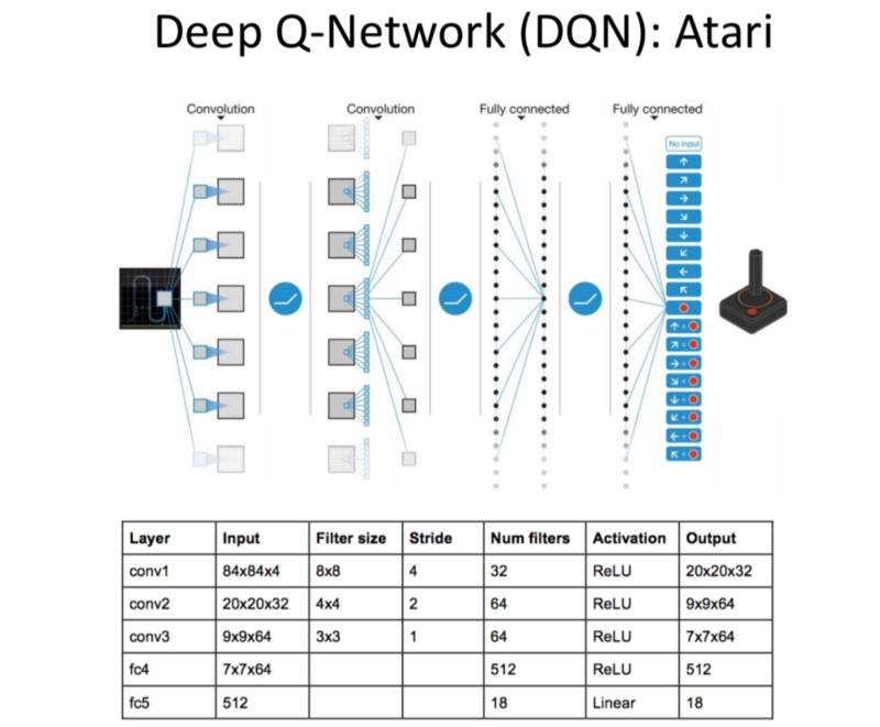
How is a DQN Trained?
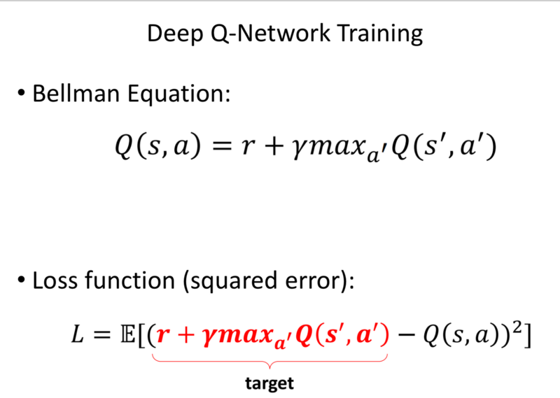
The bellman equation inputs the reward and discounts the future rewards.
Loss function for NN: takes the reward received at current state, performs a forward pass through the NN to calculate the value of future state and subtracts it from the Forward pass for the current state of action.
We take the difference between the Value estimated by Q-Function Estimator (NN) believes the future value and what the possible value will be based on the possible actions.
Algorithm:
Input: State in action
Output: Q-Value for each action.
Given a transition S, an action a that generates a reward r’ and changes to state S’.
The update is do a feed forward pass through the Netowork for the current state and do a feed forward pass for all the possible actions in the next state and update the weights using Backpropagation.
DQN Tricks:
Experience Replay:
As games are played through simulation, the observations are collected into a library of experiences and the training is performed by randomly sampling the previous experiences in batches. So that the system does not overfit a particular evolution of the simulation.
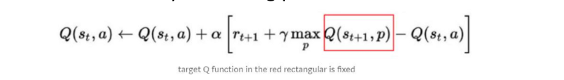
Fixed Target Network:
We use a NN to estimate the value of the current state in action-pair and the next, thereby using it multiple times. As we perform the network, we are updating the network. So the target function inside the loss function changes, which causes problems for stability. So we fix the network and only update it say, every 1,000 steps.
As we train the network, the Network used to estimate the Target function is kept fixed, resulting in a stable loss function.
Reward Clipping:
True for systems operating in generalised ways. These simplify the reward functions, to either positive or negative.
Skipping Frames:
Performing 1 action every 4 frames.
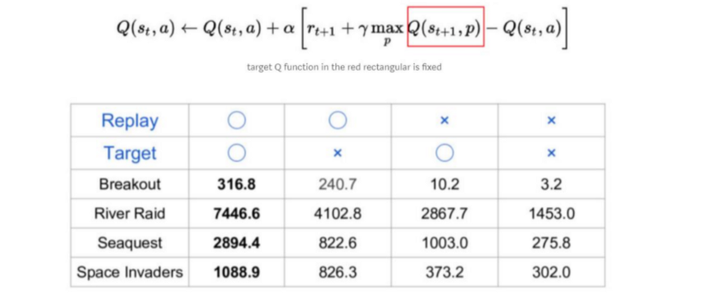
Circle: When Technique is used.
Cross: Technique not used.
Higher the number, greater the reward received.
Conclusion: Replaying Target give significant improvements for rewards.
Deep Q-Learning Algorithm:
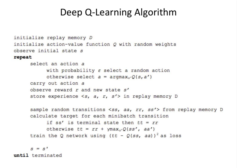
Note: The loop is not part of the training, it is the part of saving the observation, state, action, reward and next state into the replay memory.
Next we sample randomly from the memory to train the network based on a loss function. The probablity: Epsilon, is the probability of exploration-which decreases over time.
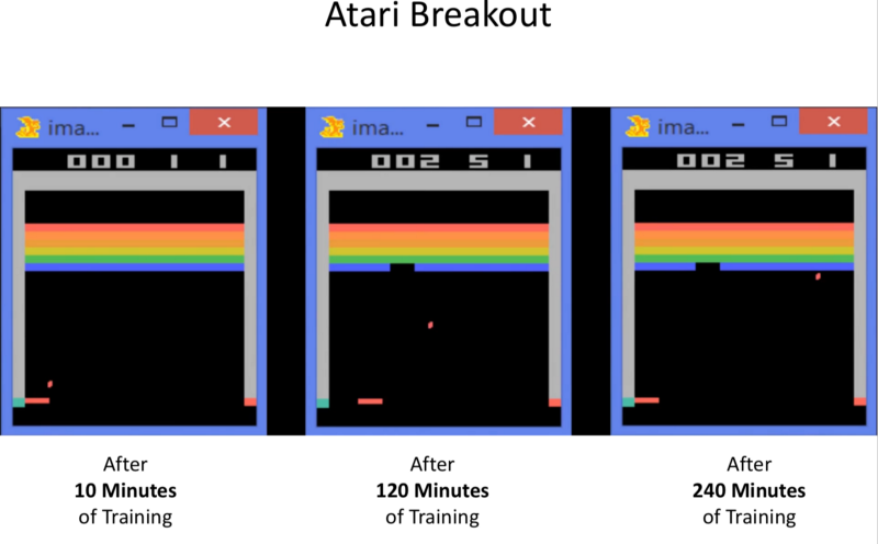
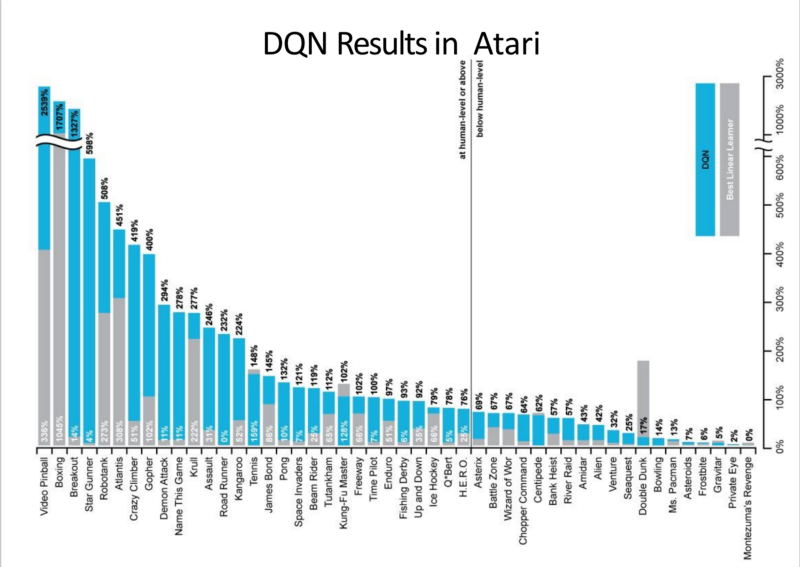
2015: Atari Breakout
DQN has outperformed on many Atari Games.
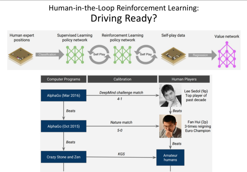
AlphaGo (2016):
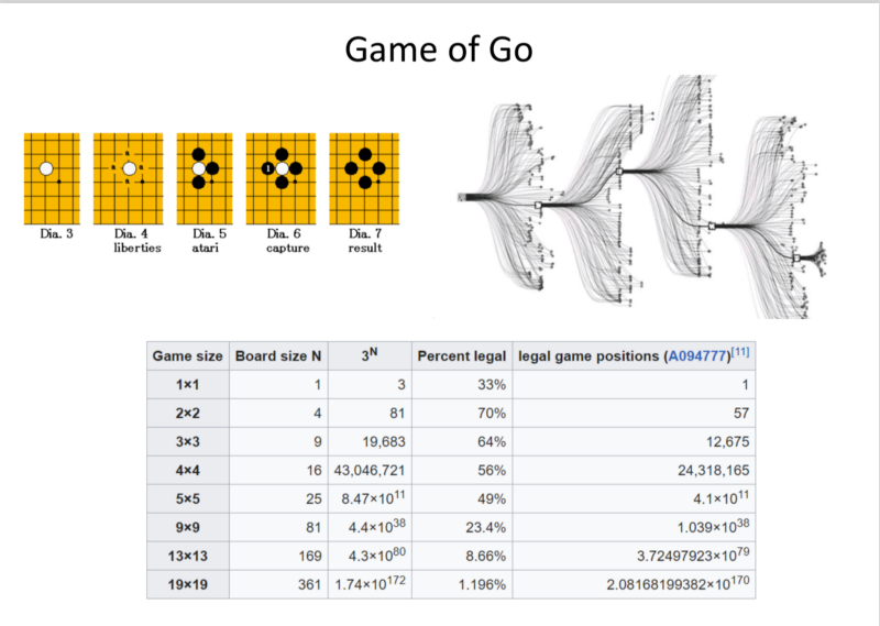
Notice: The possible legal board conditions at any point = 2.8x10^(170)
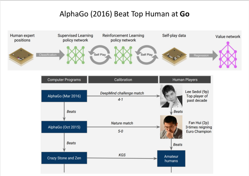
Used human expert position play to seed in a supervised way, RL approach to beat Human Experts.
(Biased) Opinion: Accomplishment of the decade in AI, AlphaGo Zero (2017):
- It was developed without any training data.
- Beat AlphaGo.
AlphaGo Approach:
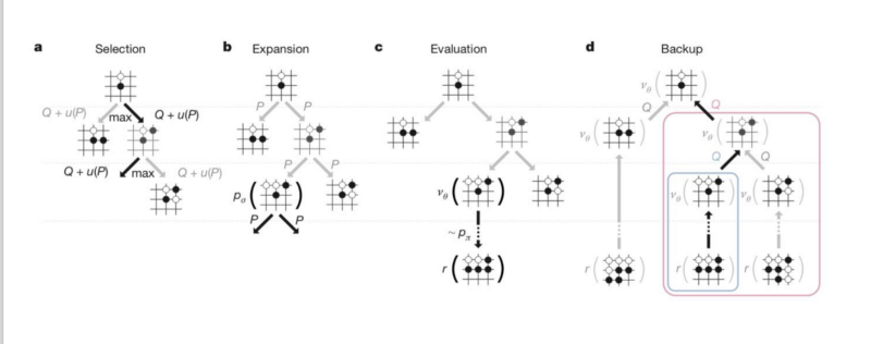
Use MTCS: Monte-Carlo Tree Search.
Given, a large state space. We start at a board, moves are chosen with some Exploration Vs Exploitation balance, until some conclusion is reached. This information is back-propagated and the we learn the value of board positions in play.
AlphGo used a Neural net for ‘Intuition’ for estimating the quality of states.
Tricks:
- Used MCTS based on NN prediction to estimate how good are the future states. It performs a simple lookahead action, does a target correction to produce loss function.
- Multi-Task Learning: The Network is “Two-Headed”,
- It outputs the probability of Optimal moves.
- It also estimates the probability of Winning.
- We want to combine the best move in short term and achieve positions with high probability of winning.
- Updated Architecture: Resnet (Winner of ImageNet)
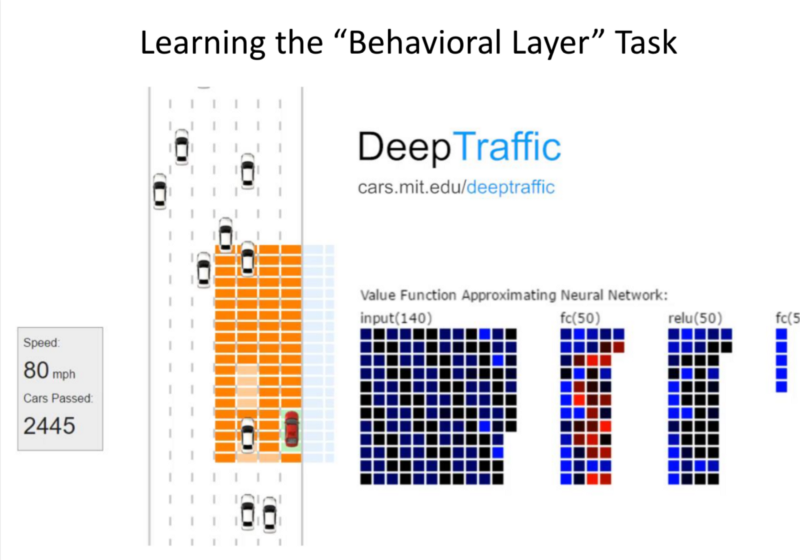
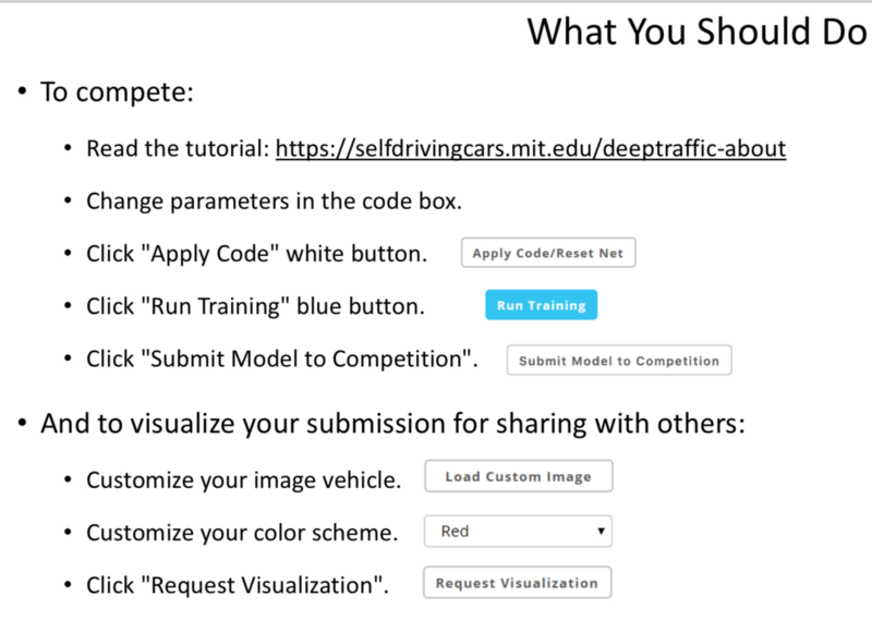
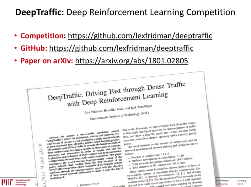
Deep Traffic
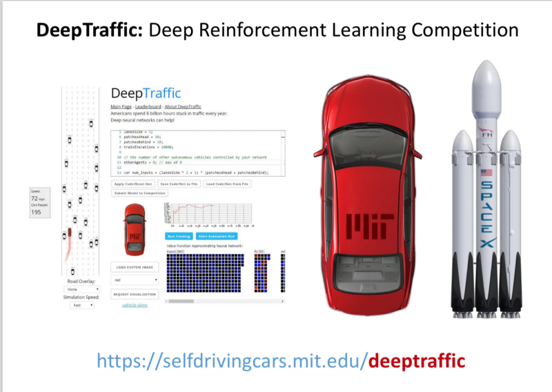
Checkout the Official Tutorial Here
v2 Features:
- We can perform multi-agent training (Upto 10 cars)
- (Cool Addition) Customising car images.
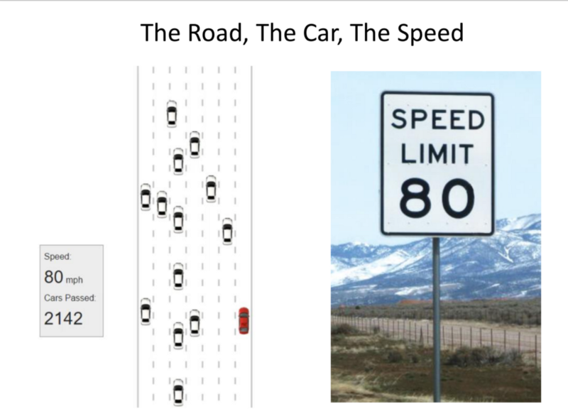
Goal: To achieve highest average speed over time.
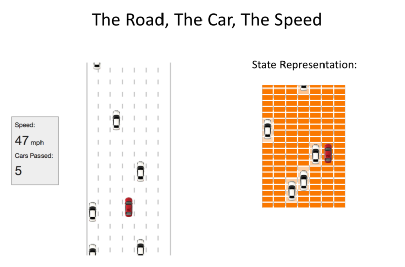
Road: Grid space, an occupancy grid: When empty, it’s set to ab-Grid value is whatever speed is achievable.
With other cars in the grid: The value in the grid is the speed of slower-moving cars.
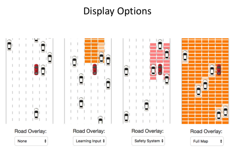
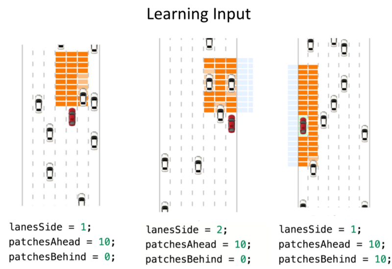
We can decide on the portion we want to use as input to the Network.
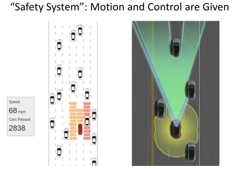
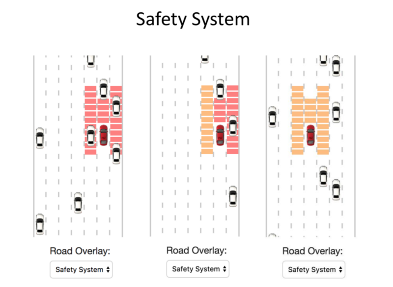
The Safety System can be considered an equivalent of Basic MPC: Basic Sensors allowing prevention of collision.
Task: To move about the space under the constraints of Safety System.
Red: Non reachable spaces.
Goal: Not get stuck in Traffic.
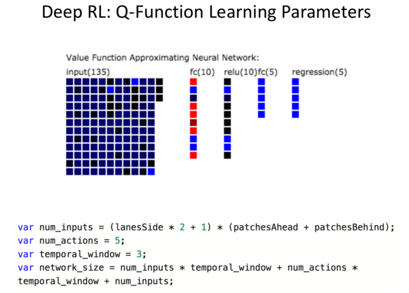
Input: State space.
Output: Value of different actions.
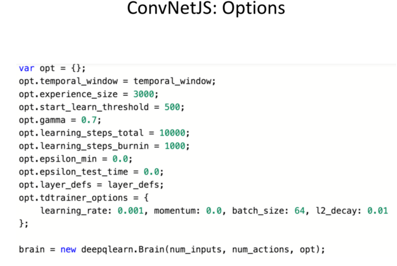
Based on Epsilon values and through training, inference evaluation: We choose exploration extent.
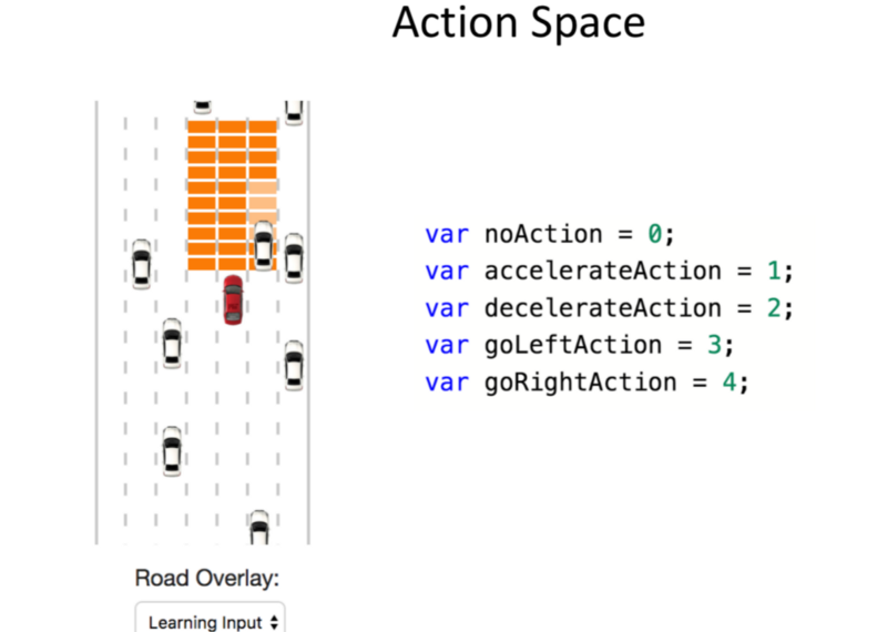
5 Action Space
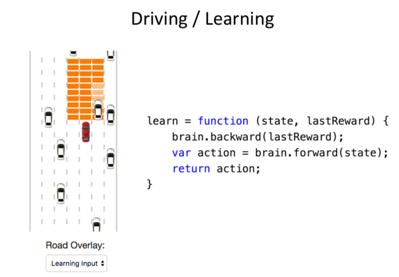
‘Brain’ takes as an input, the state. The reward performs a forward pass and calculates the reward. ‘Brain’ is where the NN is contained for both Training and Evaluation.
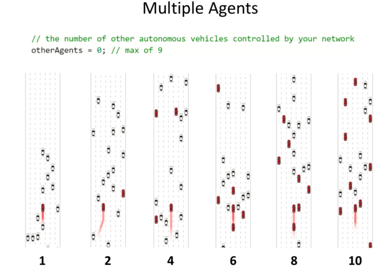
New Addition: Number of Agents that can be controlled by the NN, ranging from 1–10. The evaluation is performed in the same manner.
Note: The agents are not aware of other agent’s prescence. The actions are greedy for every individual agent and not in an optimised distributed manner.
Evaluation:
- Collecting 45 simulated seconds of each run.
- Median of 500 runs is calculated.
- Server-side evaluation.
- Randomness has been drastically reduced.
Are the RL Approach amendable to Learning with Human in the Loop?
- We can explore driver data.
- Real World Testing is not feasible.
Most Successful RL doesn’t involve Deep RL:
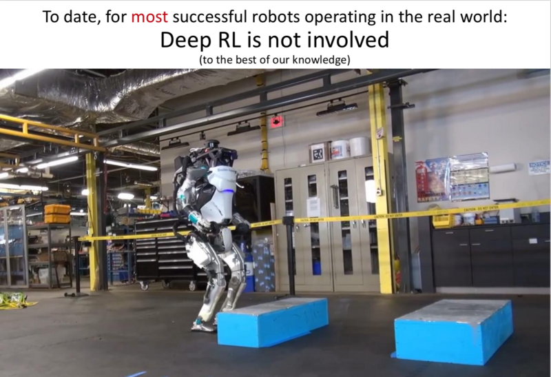
- Boston Robotics
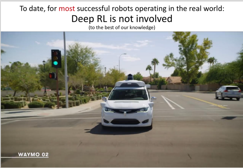
- Waymo:
DL is used in Perception.
Most of the work is done using Sensors.
Model based approaches are used.
Re: Unexpected Local Pockets of High Reward
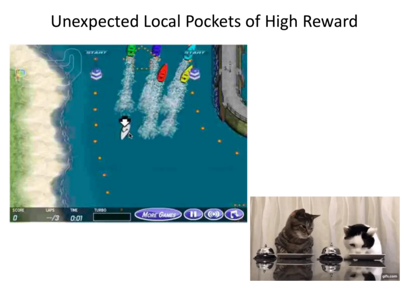
These appear in all of the examples when applied to the real world.
AI Safety:
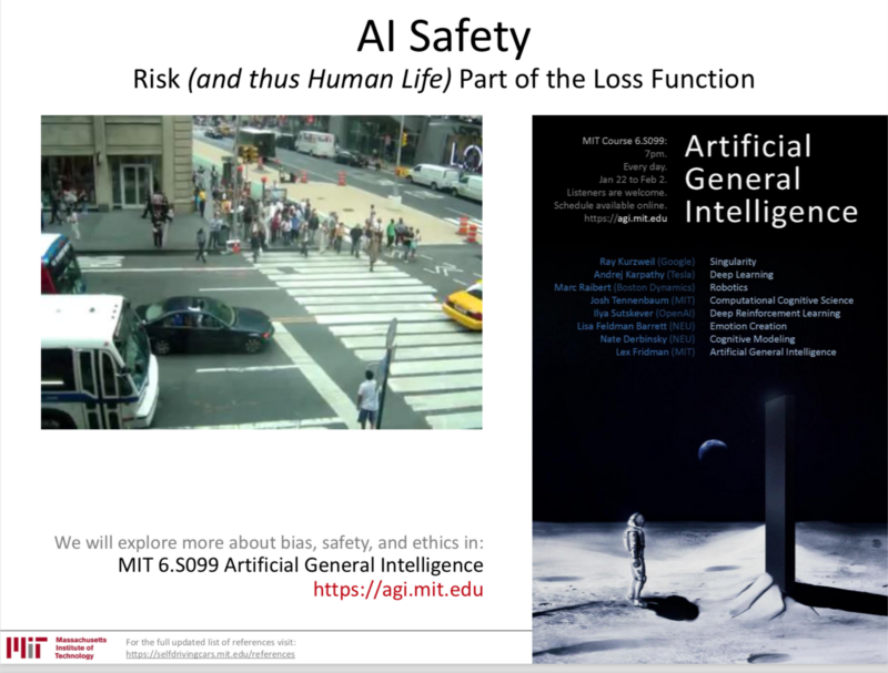
- Explore how RL Planning algorithms can evolve in unexpected ways.
- How can we constraint them? To force these to perform in a safe manner.
You can find me on twitter @bhutanisanyam1
Subscribe to my Newsletter for updates on my new posts and interviews with My Machine Learning heroes and Chai Time Data Science