

You can find all the accompanying code in this Github repo
This is Part 2 of the PyTorch Primer Series.
Linear Regression is linear approach for modeling the relationship between inputs and the predictions
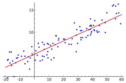
We find a ‘Linear fit’ to the data.
Fit: We are trying to predict a variable y, by fitting a curve (line here) to the data. The curve in linear regression follows a linear relationship between the scalar (x) and dependent variable.
Creating Models in PyTorch
- Create a Class
- Declare your Forward Pass
- Tune the HyperParameters
class LinearRegressionModel(nn.Module):

    def __init__(self, input_dim, output_dim):

        super(LinearRegressionModel, self).__init__()
        # Calling Super Class's constructor
        self.linear = nn.Linear(input_dim, output_dim)
        # nn.linear is defined in nn.Module

    def forward(self, x):
        # Here the forward pass is simply a linear function

        out = self.linear(x)
        return out

input_dim = 1
output_dim = 1
Steps
- Create instance of model
- Select Loss Criterion
- Choose Hyper Parameters
model = LinearRegressionModel(input_dim,output_dim)

criterion = nn.MSELoss()# Mean Squared Loss
l_rate = 0.01
optimiser = torch.optim.SGD(model.parameters(), lr = l_rate) #Stochastic Gradient Descent

epochs = 2000
Training The Model
for epoch in range(epochs):

    epoch +=1
    #increase the number of epochs by 1 every time

    inputs = Variable(torch.from_numpy(x_train))
    labels = Variable(torch.from_numpy(y_correct))

    #clear grads as discussed in prev post

    optimiser.zero_grad()

    #forward to get predicted values

    outputs = model.forward(inputs)
    loss = criterion(outputs, labels)
    loss.backward()# back props
    optimiser.step()# update the parameters
    print('epoch {}, loss {}'.format(epoch,loss.data[0]))
Finally, Print the Predicted Values
predicted =model.forward(Variable(torch.from_numpy(x_train))).data.numpy()

plt.plot(x_train, y_correct, 'go', label = 'from data', alpha = .5)
plt.plot(x_train, predicted, label = 'prediction', alpha = 0.5)
plt.legend()
plt.show()
print(model.state_dict())
If you want to read about Week 2 in my Self Driving Journey, here is the blog post
The Next Part in the Series will discuss about Linear Regression.
You can find me on twitter @bhutanisanyam1
Subscribe to my Newsletter for updates on my new posts and interviews with My Machine Learning heroes and Chai Time Data Science